How do algorithms listen to music?

From copyright monitoring and cover song detection to classifications of all kinds (genre, style, mood, key, year, epoch), all the way to the music curation war waged by the music streaming titans, music identification is a major component in today’s music industry and society at large. Alongside Shazam and its worldwide popularity, a myriad of other algorithms have emerged in the past two decades, each with its own strengths and weaknesses. In this article, we’ll take you for an overview tour of the different approaches to identifying a song or songs based on an audio file, following what’s called the “query-by-example” (QBE) paradigm.

Identifying a track: Shazam’s modus operandi

First and foremost, let’s introduce the concept of specificity, which indicates the degree of similarity between the audio extract and the result(s) put forward by the algorithm. For example, exact duplicates exhibit the highest specificity there is, whereas a song and its cover generally offer a mid-specific match, with a degree of similarity that depends on numerous parameters. In this first approach, the goal is to identify the precise track that’s being played back by using a high-specificity matching algorithm to compare the audio excerpt’s “fingerprint” to those of the songs in the database.

Let’s look at a typical Shazam use. Most of the time the query will be nothing more than an audio fragment, never recorded from the top of the song, very likely affected by noise, and sometimes even altered by compression (data/dynamics) and/or equalization. But to be reliably identified, its fingerprint must remain robust against such alterations of the original signal, all while being compact and efficiently computable so as to optimize storage space and transmission speed.

To understand Shazam’s process, based on Avery Li-Chun Wang’s research, let’s follow the song’s journey. Once the audio fragment is captured by a smartphone’s microphone(s), the app generates a spectrogram of the song — a representation of the frequencies and their magnitude (volume) as they vary over time. Then the app extracts the locally loudest points to create what is called a constellation map, exclusively composed of frequency-time peaks.

Anchor frequency-time peak (red); target frequency-time peaks (green)

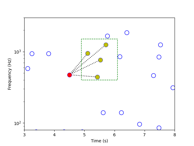
The app then chooses a peak to serve as an “anchor peak,” and chooses a “target zone” as well. Pairing each peak in the target zone with the anchor peak creates “hash values,” a triplet composed of both frequency values and the time difference between the peaks. The hash values approach has significant advantages over comparing the song’s constellation map to all constellation maps in the database: it’s time-translation-invariant (that is, there’s no absolute time reference, only relative time differences); it’s more efficiently matchable against the database fingerprints; and it’s more robust against signal distortions. It is also much more specific, which allows the query to be a very short fragment of the original piece, thus allowing the app to deliver a quick result to the user.

Shazam’s identification is so specific that it can catch a playback singer pretending to perform live: if the app identifies the studio version of a song during a concert, it means the exact original recording is being played back, down to a quarter tone and a sixteenth note. However, its main weakness is precisely the other side of the specificity coin: unless the song is the exact same studio recording itself, the algorithm is completely unable to identify it, even if performed by the same artist, in the same key, at the same tempo as the original song or remix. Which leads us to our second approach.

Identifying a song: a study in chroma

This time around, the algorithm must identify a song rather than a precise track, whether it is the original studio recording, a remix, or a live version of it. This means the audio fragment needs contain certain invariant properties of a particular recording.

Comparison between two spectrogram-based constellation maps: Michael Jackson’s studio version of “Beat It” (left) and his live performance of it in Auckland (right)

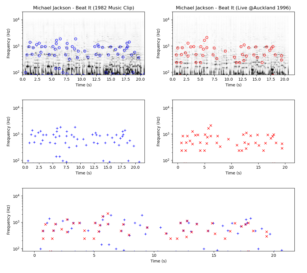
For instance, here’s the peak-based fingerprint comparison between the original recording of Beat It, and Michael Jackson’s live performance at Auckland in 1996: as you can see, although the artist and the key are left unchanged, the two spectrogram-based constellations are not a perfect match. Enter the chromagram: this representation doesn’t show the precise frequency decomposition (which not only includes the pitch, but also the timbre) as a function of time, but rather captures the  harmonic progression and the melodic characteristics of the excerpt. In other words, it delivers a much more musical description. Assuming an equal-tempered scale, the music pitches are categorized in chroma bins — usually twelve, which represent the twelve pitch classes (C, C♯, D, D♯, … , B) of Western tonal music.

There are many ways to extract the chroma features of an audio file, and these features can be further sharpened with suitable pre- and post-processing techniques (spectral, temporal, and dynamic) in order to produce certain types of results (more or less robust to tempo, interpretation, instrumentation, and many other types of variations).

Instead of comparing hash values, whole sub-sequences of the chroma features are compared to the database’s complete chromagrams. The matching process is therefore much slower than with spectrogram fingerprinting. In short, while the chroma-based approach is great for retrieving remixes or remasters and for detecting covers, thanks to its strong robustness to changes in timbre, tempo and instrumentation, it is only suitable for medium size databases — and of course doesn’t offer the same level of precision as audio identification.

Identifying a version: the matrix

In this last section, we’ll allow the degree of specificity to sink even lower: here, given an audio query, the goal is to fetch any existing rearrangements of a song, no matter how different it is from the original piece. Let’s take Imagine, by John Lennon & The Plastic Ono Band: what do you think of this version? A pretty simple modal change, from major to minor, and the lyrics take on a whole different meaning — which raises the question of a composition’s boundaries: would you consider this a cover, or an entirely different song?

Besides mode (and obviously, timbre), a cover may differ from the initial composition in many ways, such as tonality, harmony, melody, rhythmic signature, and even lyrics. Let’s go back to our first example, and compare the studio recording of Beat It with its reinterpretation by Fall Out Boy:

Similarity matrix between Michael Jackson’s “Beat It” and Fall Out Boy’s cover.

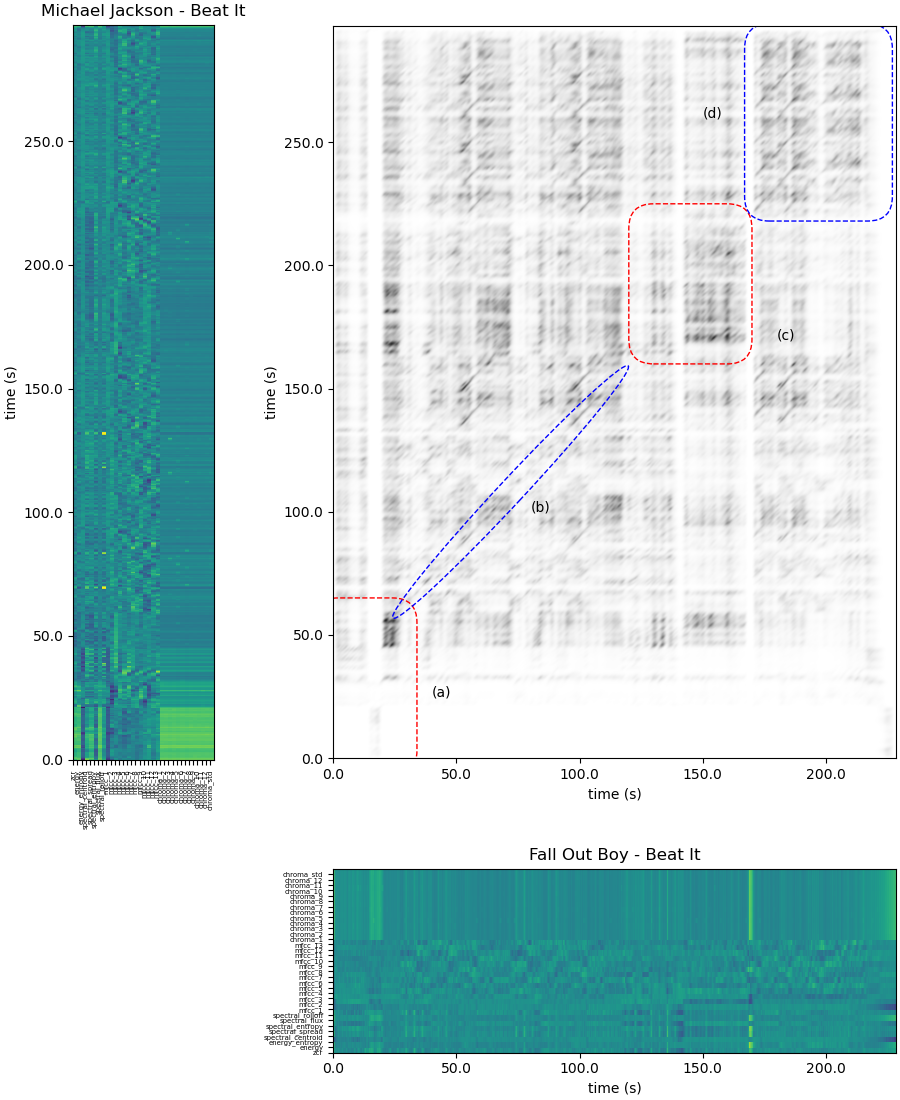
What you can see above is called a similarity matrix, which offers pairwise similarity between the query and any audio file: high similarities appear in the form of diagonal paths. While this type of matrix is partly based on chroma vectors, it also uses a whole set of indicators, including entropy of energy, spectral spread, and zero crossing rate, among others (you can find the detailed list here). Let’s take a closer look at this particular similarity matrix — and while reading our explanations, feel free to compare the two songs by ear.

The (a) zone exhibits no diagonals, which shows that the two songs’ intros are very different with respect to structure as well as to sounds, harmony, and melody. The (b) zone, however, exhibits clear diagonal lines, which indicate a good correlation and therefore clear similarities between the two versions during the first verse, the first chorus, the second verse and the second chorus of the song. In the (c) zone — that is, the bridge — while temporal correlation is poor, small diagonal patches appear due to the presence of a guitar solo in both versions. Finally, the correlation at the end of the song (repetition of the chorus) is illustrated by the return of the diagonal paths.

To determine if two audio clips are musically related, a so-called accumulated score matrix indicates the length and quality of the correlated parts based on the similarity matrix’s results, and takes into account specific penalties. The final score is then used for ranking the results for a given query, from most to least similar.

As you can imagine, that kind of music retrieval mechanism constitutes a particularly cost-intensive approach. Actually, one could simply sum up this paper by saying “the lower the specificity, the higher the complexity,” because when dealing with music collections comprising millions of songs, mid- and low-specific algorithms still raise myriad unanswered questions. In the future, these complementary approaches could be combined to offer a much more flexible experience: one could imagine an app which would allow the user to adjust the degree of similarity they’re looking for, select a particular part of the song — the whole piece or just a snippet — and even indicate the musical properties they need the algorithm to focus on. Here’s hoping!

All the illustrations were created using the open-source Python library for audio signal analysis developed by Theodoros Giannakopoulos.

Sources:
Similarity matrix processing for music structure analysis, by Yu Shiu, Hong Jeong and C.-C. Jay Kuo
Audio content-based music retrieval, by Peter Grosche, Meinard Müller and Joan Serrà
Visualizing music and audio using self-similarity, by Jonathan Foote
Cover song identification with 2D Fourier transform sequences, by Prem Seetharaman and Zafar Rafii